Statistical Reasoning and Its Application in Real Life

Using collaborative activities, task learners to discuss the concepts mean, median and mode and how to obtain them by dwelling on ideas from JHS. Then, solve some problems to consolidate their ideas on these concepts - mean, median and mode for grouped data.
Example 1: Mode for grouped data is found using the following mode formula.

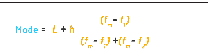
Where:
- L is the lower limit of the modal class.
- 'h' is the size of the class interval.
- 'fm' is the frequency of the modal class.
- 'f1' is the frequency of the class preceding the modal class.
- 'f2' is the frequency of the class succeeding the modal class.
The median formula for grouped data is given as, 𝒏𝒏 − 𝑭𝑭 𝒎𝒎𝒎𝒎𝒎𝒎𝒎𝒎𝒎𝒎𝒎𝒎 = 𝑳𝑳 𝒎𝒎 + [ 𝟐𝟐 ] 𝒊𝒊 𝑭𝑭 𝒎𝒎
Where: n = total frequency F = cumulative frequency F m = frequency of other class median I= class width L m = lower boundary of the class median
Similarly, we have a mean formula for grouped data. Which is expressed as: ∑ 𝑓𝑓𝑓𝑓 𝑚𝑚𝑚𝑚𝑚𝑚𝑚𝑚 = ∑𝑓𝑓 Where: ∑ = is the summation sign x = the mean value of the set of given data. f = frequency of the individual data
Example 2: Establish the relation between mean, median and mode.
The three measures of central values, i.e., mean, median, and mode, are closely connected by the following relations (called an empirical relationship). 2Mean + Mode = 3Median For example, we have data whose mode = 65 and median = 61.6. Then, we can find the mean using the above mean, median, and mode relation. 2Mean + Mode = 3 Median ∴2Mean = 3 × 61.6 - 65 ∴2Mean = 119.8 ⇒ Mean = 119.8/2 ⇒ Mean = 59.9
Example 3: Establish that the mean is a form of average The term average is frequently used in everyday life to denote a value that is typical for a group of quantities. Average rainfall in a month or the average age of employees of an Organisation is a typical example.
- Average is the value that indicates what is most likely to be expected.
- They help to summarise large data into a single value.
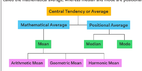
An average tends to lie centrally with the values of the observations arranged in ascending order of magnitude. So, we call it an average measure of the central tendency of the data. Averages are of different types. What we refer to as mean, i.e., the arithmetic mean, is one of the averages. Mean is called the mathematical average, whereas median and mode are positional averages. 

Using collaborative activities, task learners on the difference between mean and median.
Example: A department of an Organisation has 5 employees, which include a supervisor and four executives. The executives draw a salary of GH 10,000 per month, while the supervisor gets GH 40,000.
Solution: Mean = (10000 + 10000 + 10000 + 10000 + 40000)/5 = 80000/5 = 16000 Thus, the mean salary is GH 16,000.
To find the median, we consider the ascending order: 10000, 10000, 10000, 10000, 40000. n = 5, so, (n + 1)/2 = 3 Thus, the median is the 3rd observation. Median = GH10,000
Thus, the median is GH10,000 per month.
Now, let us compare the two measures of central tendencies. We can observe that the mean salary of GH 16,000 does not give even an estimated salary of any of the employees, whereas the median salary represents the data more effectively. One of the weaknesses of the mean is that it gets affected by extreme values.
Using collaborative activities, task learners to discuss the effect of an extreme value on the mean.
Example: The following graph shows how extreme values affect mean and median:

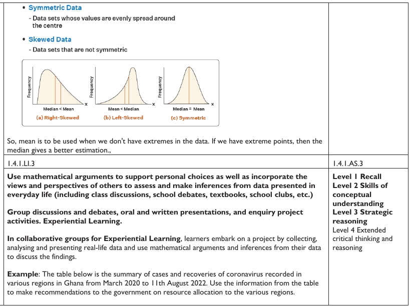
So, mean is to be used when we don't have extremes in the data. If we have extreme points, then the median gives a better estimation.,
Teaching and Learning Resources:
- * Graph sheets * mathematical sets * computer with data organising software like MS Excel, MS
- PowerPoint, etc. * A4, A3 papers * flip charts
- * markers * colour pens, etc. * Reports from analysed data * manila cards
- * worksheets * posters * teaching presentations * enquiry project-template
Assessment (1.4.1.AS.2). The document marks these depth-of-knowledge levels for this indicator: Level 1 Recall; Level 2 Skills of conceptual understanding; Level 3 Strategic reasoning; Level 4 Extended critical thinking and reasoning.