SHS3 Mathematics · Semester 2, Week 7
Measurement
Full lesson notes coming
Notes for this lesson are being prepared. The curriculum details below are complete and ready to use for your planning.
Curriculum details
- Strand
- Geometry Around Us (Strand 3)
- Sub-strand
- Measurement (3.2)
- Content standard
- 3.3.2.CS.1 - Demonstrate conceptual understanding of trigonometric graphs and use them to solve trigonometric equations. 3.3.2.LO.1 Draw graphs of given trigonometric functions and use them to determine equations and solve related problems.
- Indicator
- 3.3.2.LI.1 - Draw graphs of given trigonometric functions and use them to solve related problems.
- Suggested placement
-
Semester 2, Week 7
(Week 27 of the year)
Our suggestion, laid out in curriculum order across three terms of twelve weeks. NaCCA does not fix the week, so follow your school's scheme of learning.
- Source document note
-
The official curriculum document has a fault in this entry, so the curriculum text above is transcribed exactly as printed:
- exemplars - p.361: this exemplar sets a two-dimensional construct - a stacked fraction, an index or a column vector - which the text layer flattens into separate lines, so the parts are present but their vertical arrangement is lost; read the page
- Curriculum reference
- NaCCA curriculum document, p. 356
Exemplars (from the NaCCA curriculum)
Group discussion: Learners discuss Sine, Cosine and Tangent graphs with examples. Encourage learners to behave and work in a controlled way, which involves obeying mathematical rules, principles and standards, leading to self-directed learning.
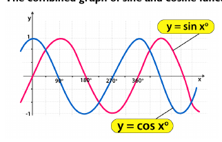
Example 1 What is the plot of sin? The Sine Function has this beautiful up-down curve (which repeats every 2π radians, or 360°). It starts at 0, heads up to 1 by π/2 radians (90°) and then heads down to −1.
What is the plot of cosine? Cosine is just like Sine, but it starts at 1 and heads down until π radians (180°) and then heads up again.

The combined graph of sine and cosine functions can be represented as follows.
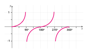
What is the plot of the tangent? The Tangent function has a completely different shape ... it goes between negative and positive Infinity, crossing through 0 and at every π radian (180°), as shown on this plot. At π/2 radians (90°), and at −π/2 (−90°), 3π/2 (270°), etc., the function is officially undefined because it could be positive Infinity or negative Infinity.
Example 2:
i. Sketch the graph of the sine function on the interval [𝟎, 𝟒𝝅] and find the range.
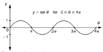
The range of 𝑦 = sin 𝜃 is −1 ≤ 𝑦 ≤ 1 .
ii. Sketch the graph of the sine function on the interval (−𝟐𝝅, 𝟐𝝅).

iii. Sketch the graph of the cosine function on the interval (𝟎, 𝟒𝝅).
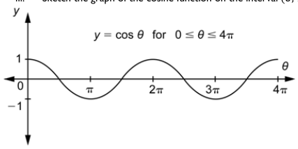
v. Sketch the graph of the cosine function on the interval (−𝟐𝝅, 𝟐𝝅).
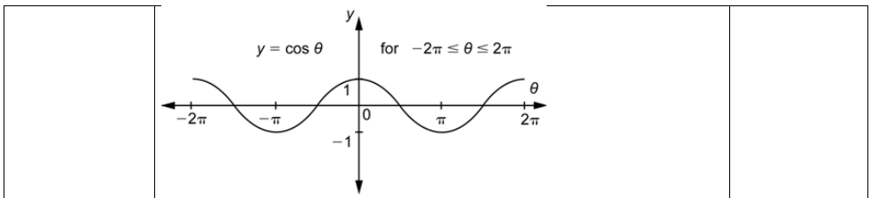
A Comparison of the Graphs of Sine and Cosine The graphs of sine and cosine both have hills and valleys in a repeating pattern. Since this repeating pattern can be extended indefinitely to the left and right, the domain for both functions is the real numbers. The range for both of them is the interval.
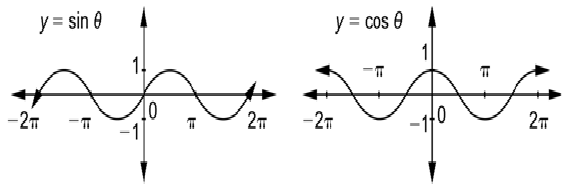
Group discussions: Learners draw sine, cosine and tangent graphs. Engage learners in the development of healthy and supportive relationships with their peers as they communicate with diverse individuals in their groups.
Plotting a cosine graph
Examples: i. Sketch the graph of Y = f(θ) = cos θ [0° ≤ θ ≤ 360°]. Use your calculator to complete the following table. Choose an appropriate scale and plot the values of θ on the x-axis and cos θ on the y-axis. Round your answers to 2 decimal places.
𝜃 0 0 30 0 60 0 90 0 120 0 150 0 180 0 210 0 270 300 0 330 0 360 0
cos 𝜃
Solution Step 1: Substitute values for 𝜽. 𝜃 0 0 30 0 60 0 90 0 120 0 150 0 180 0 210 0 240 270 0 300 0 330 0 360 0 cos 𝜃 1 0.87 0.5 0 -0.5 - -1 - - 0 0.5 0.87 1 0.87 0.87 0.5
Step 2: Plot the points and join with a smooth curve
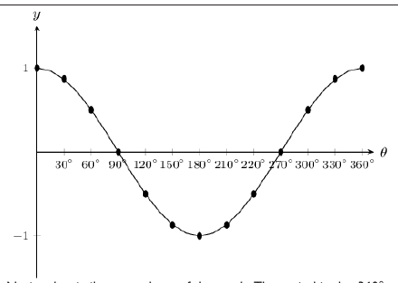
Notice the similar wave shape of the graph. The period is also 360°, and the amplitude is 1. The maximum value of y = cos θ is 1, and the minimum value is −1.
Domain: [0°; 360°] Range: [−1; 1] x-intercepts: (90°; 0), (270°; 0) Y: (0°; 1) Maximum turning points: (0°; 1), (360°; 1) Minimum turning point: (180°; −1)
Sketch the graph of f(θ) = 2 sin θ + 3 for θ ∈ [0°; 360°]. ii. Step 1: Examine the standard form of the equation: From the equation, we see that a > 1, so the graph is stretched vertically. We also see that q > 0, so the graph is shifted vertically upwards by 3 units. Step 2: Substitute values for θ:

𝜃 0 0 30 0 60 0 90 0 120 0 150 0 180 0 210 0 240 0 270 0 300 0 330 0 360 0

 𝑓( 𝜃) 3 4 4.73 5 4.73 4 3 2 1.27 1 1.27 2 3
Step 3: Plot the points and join with a smooth curve
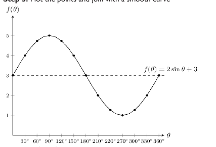
Domain: [0°;360°] Range: [1;5] x-intercepts: none y-intercepts: (0°;3) Maximum turning point: (90°;5) Minimum turning point: (270°;1)
iii. Plotting a tangent graph Sketch the graph of Y = f(θ) = tan θ [0° ≤ θ ≤ 360°] Use your calculator to complete the following table. Choose an appropriate scale and plot the values with θ on the x-axis and tan θ on the y-axis. Round your answers to 2 decimal places.
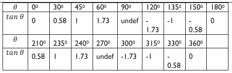
 𝜃 0 0 30 0 45 0 60 0 90 0 120 0 135 0 150 0 180 0 𝑡𝑎𝑛 𝜃 0 0.58 1 1.73 undef - -1 - 0 1.73 0.58 𝜃 210 0 235 0 240 0 270 0 300 0 315 0 330 0 360 0 𝑡𝑎𝑛 𝜃 0.58 1 1.73 undef -1.73 -1 - 0 0.58
Plot the points and join them with a smooth curve.
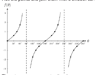
There is an easy way to visualise the tangent graph. Consider our definitions of sin θ and cos θ for right-angled triangles: So, for any value of θ: 𝑠𝑖𝑛𝜃 Tan θ = 𝑐𝑜𝑠𝜃
So, we know that for values of θ for which sin θ = 0, we must also have tan θ = 0. Also, if cos θ = 0, the value of tan θ is undefined as we cannot divide by 0. The dashed vertical lines are at the values of θ where tan θ is not defined and are called the asymptotes. Asymptotes: the lines θ = 90° and θ = 270° Period: 180°
Domain: {θ: 0° ≤ θ ≤ 360°,θ ≠ 90°; 270°} Range: {f(θ) : f(θ) ∈R} x-intercepts: (0°;0), (180°;0), (360°;0) y-intercept: (0°;0)
Teaching and Learning Resources:
- Mathematical sets, Graph sheet.
- Technology tools such as computers, mobile phones, etc.
- Computer software applications like GeoGebra.
Assessment (3.3.2.AS.1). The document marks these depth-of-knowledge levels for this indicator: Level 2 Skills of conceptual understanding.