SHS1 Additional Mathematics · Semester 2, Week 15
Organising, Representing and Interpreting Data
Full lesson notes coming
Notes for this lesson are being prepared. The curriculum details below are complete and ready to use for your planning.
Curriculum details
- Strand
- Handling Data (Strand 4)
- Sub-strand
- Organising, Representing and Interpreting Data (4.1)
- Content standard
- 1.4.1.CS.1 - Investigate techniques for collecting data and determine measures of central tendency and dispersion. 1.4.1.LO.1 Collect quantitative and qualitative data, and organise and present data using graphs. 1.4.1.LO.2 Calculate the measures of central tendencies, and measures of dispersion and use simple language to interpret the results.
- Indicator
- 1.4.1.LI.5 - Present grouped data using appropriate graphs by hand and/or by appropriate technology and justify why a particular representation is more suitable than others for a given situation.
- Suggested placement
-
Semester 2, Week 15
(Week 35 of the year)
Our suggestion, laid out in curriculum order across three terms of twelve weeks. NaCCA does not fix the week, so follow your school's scheme of learning.
- Source document note
-
The official curriculum document has a fault in this entry, so the curriculum text above is transcribed exactly as printed:
- exemplars - p.223: adjacent duplicated CambriaMath characters were collapsed, but this PDF also maps some equation glyphs to the wrong letter or operator; verify every mathematical expression in this row against the rendered page
- exemplars - p.224: a stacked fraction, matrix, vector or other two-dimensional construct is flattened by the text layer; all visible parts require comparison with the rendered page
- Curriculum reference
- NaCCA curriculum document, p. 223
Exemplars (from the NaCCA curriculum)
Group discussions, Talk for Learning, experiential learning, building on what others say.
Learning Experience: Learners in mixed-ability groups discuss how to represent data using histograms and cumulative curves.
Activity 1:
- Learners in groups recall how to represent data using histogram with equal intervals.
- Learners in groups collaborate and solve practical questions by representing data using a histogram with equal intervals.
- Learners recollect how to estimate the measures of central tendencies using the histogram.
Activity 2:
- Learners in their groups brainstorm to discover how to represent data using a histogram with unequal intervals.
- Learners in groups recognise that data given for such histograms have unequal intervals.
Example 1: 1-5, 5-15, 15-20, 20-35 etc.
- Learners in groups discover that in order to represent data with unequal intervals, it is necessary for the area of each bar in a histogram, rather than the height, to represent the frequency.
- Learners discover that to draw a histogram for unequal class intervals, you need to adjust the heights of the bars so the area is proportional to the frequency.
NOTE: The height of the bar, called the frequency density, is found by dividing the frequency by the g3N`XN%;A class width, i.e. 𝑓 𝑑 = ;_&OO hL<GW
- Learners solve a practical example of data with unequal intervals.
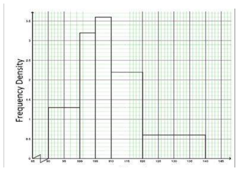
Example 1: The table gives information about the speed of cars in 𝑘/ℎ of 81 cars
Speed(s) 𝑘/ℎ Frequency 90 < 𝑠 ≤ 100 13 100 < 𝑠 ≤ 105 16 105 < 𝑠 ≤ 110 18 110 < 𝑠 ≤ 120 22 120 < 𝑠 ≤ 140 12
Draw a histogram to represent the information in the table.
Solution: Frequency table
Speed Class Frequency Class Frequency boundaries width density 90 < 𝑠 90 13 10 1.3 ≤ 100 100 < 𝑠 100 16 5 3.2 ≤ 105
105 < 𝑠 105 18 5 3.6 ≤ 110 110 < 𝑠 110 22 10 2.2 ≤ 120 120 < 𝑠 120 12 20 0.6 ≤ 140
- Learners in groups create practical examples and solve them in their various groups.
Activity 3:
- Learners in their collaborative groups construct cumulative frequency curves (ogive) to represent data.
- Learners in their collaborative groups recollect how to construct cumulative frequencies to represent data.
- Learners solve practical examples.
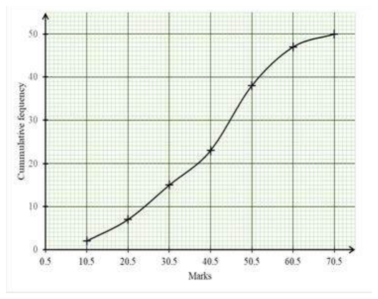
Example 1: The distribution of marks for 50 students in a test is given in the table. Draw a cumulative frequency curve to the distribution.
Marks Frequency 1-10 2 11-20 5 21-30 8 31-40 8 41-50 15 51-60 9 61-70 3
Teaching and Learning Resources:
- SHS curriculum
- Research journals
- Internet or e-books
- Real-life examples
- Software (Excel, SPSS)
Assessment (1.4.1.AS.5). The document marks these depth-of-knowledge levels for this indicator: Level 4 Extended critical thinking and reasoning.