Statistical Reasoning and Its Application in Real Life

Using Talk for Learning strategies, learners brainstorm on the meaning of standard deviation.
Example: Standard deviation tells about the value and how much it has deviated from the mean value. If we get a low standard deviation, then it means that the values tend to be close to the mean, whereas a high standard deviation tells us that the values are far from the mean value. It is commonly abbreviated as SD and denoted by 'σ'.
Using think-pair-share activities, learners discuss the steps in determining standard deviation and deduce the formula for Standard deviation.
Steps to Calculate Standard Deviation
- Find the mean, which is the arithmetic mean of the observations.
- Find the squared differences from the mean. (The data value - mean) 2
- Find the average of the squared differences. (Variance = The sum of squared differences ÷ the number of observations).
- Find the square root of variance. (Standard deviation = √Variance).
Standard Deviation Formulae: Two standard deviation formulas are used to find the standard deviation of sample data and the standard deviation of the given population. 

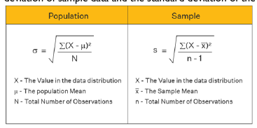
Standard Deviation of Ungrouped Data: The calculations for standard deviation differ for different data. Distribution measures the deviation of data from its mean or average position. There are two methods to find the standard deviation.
Standard Deviation by the Actual Mean Method σ = √(∑x−¯x)2/n)
Example: Consider the data observations 3, 2, 5, 6. Here, the mean of these data points is 16/4 = 4. The squared differences from mean = (4-3) 2 +(2-4) 2 +(5-4) 2 +(6-4) 2 = 10 Variance = Squared differences from mean/ number of data points =10/4 =2.5 Standard deviation = √2.5 = 1.58.
Standard deviation by Assumed Mean Method: When the x values are large, an arbitrary value (A) is chosen as the mean. The deviation from this assumed mean is calculated as d = x - A.
σ = √[(∑(d) 2 /n) - (∑d/n) 2 ]
Using Talk for Learning: Learners brainstorm on the meaning of variance.
Example: Variance is a measure of dispersion. A measure of dispersion is a quantity that is used to check the variability of data about an average value. Data can be of two types - grouped and ungrouped. When data is expressed in the form of class intervals, it is known as grouped data. On the other hand, if data consists of individual data points, it is called ungrouped data. The sample and population variance can be determined for both kinds of data.
Using think-pair-share activities, learners discuss the steps in determining variance and deduce the formula for variance. Learners should be encouraged to use feasible technology to analyse data, determine the variance of the data, and talk about the appropriate ways of using the IT tools.
Example
- Find the mean of the observations.
- Subtract the mean from each observation.
- Square each of these values.
- Add all the values obtained in the previous step.
- Divide the value from step 4 by n (for population variance) or n - 1 (for sample variance). 

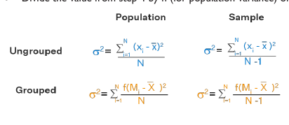
Examples: i. Suppose we have the data set {3, 5, 8, 1}, and we want to find the population variance. The mean is given as (3 + 5 + 8 + 1) / 4 = 4.25. Then by using the definition of variance we get [(3 - 4.25) 2 + (5 - 4.25) 2 + (8 - 4.25) 2 + (1 - 4.25) 2 ] / 4 = 6.68. Thus, variance = 6.68.
ii. Find the sample variance of the data (3, 4, 7, 12, 14).
Solution: n = 5 Mean = (3 + 4 + 7 + 12 + 14) / 5 = 8 Sample Variance = ∑(Xi−𝑋̅ ) 2 /N−1 [(3 - 8) 2 + (4 - 8) 2 + (7 - 8) 2 + (12 - 8) 2 + (14 - 8) 2 ) / 5 - 1 = 23.5
Answer: Variance = 23.5
iii. Find the population variance of the data (1.2, 4.5, 6.7, 2.3).
Solution: n = 4 Mean = (1.2 + 4.5 + 6.7 + 2.3) / 4 = 3.675 Population Variance = ∑(Xi−X) 2 /N [(1.2 - 3.675) 2 + (4.5 - 3.675) 2 + (6.7 - 3.675) 2 + (2.3 - 3.675) 2 ] / 4 = 4.461
Answer: Variance = 4.461
iv. Find the sample variance of Class 10 - 20 - 30 - 40 - 50 - 20 30 40 50 60
Frequency 2 5 7 3 1
Solution: The height of the interval is 10 Class F Mi d = (Mi - fd d 2 f B) / 10 10 - 20 2 15 -2 -4 8 20 - 30 5 25 -1 -5 5 30 - 40 7 35 = 0 0 0 B 40 - 50 3 45 1 3 3 50 - 60 1 55 2 2 4
∑𝑀𝑀𝑀𝑀𝑀𝑀𝑀𝑀 Mean = = 32.778. ∑𝑓𝑓𝑓𝑓
(∑𝑓𝑓𝑓𝑓) ∑𝑓𝑓𝑑𝑑 2 − Variance = 2𝑛𝑛 .10 2 = 112.4183. [This formula can be derived from ∑f(Mi−¯¯¯¯¯X)2N−1 to 𝑛𝑛−1 simplify calculations] Answer: Variance = 112.4183.
Using Talk for Learning: Learners brainstorm on the meaning of Quartile Deviation.
Example: Quartile deviation is a statistic that measures the deviation in the middle of the data. Quartile deviation is also referred to as the semi-interquartile range and is half of the difference between the third quartile and the first quartile value. The formula for the quartile deviation of the data is 

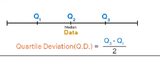
Examples: Find the quartile deviation for the following given data. 23, 8, 5, 16, 33, 7, 24, 5, 30, 33, 37, 30, 9, 11, 26, 32
Solution: The given data points are 23, 8, 5, 16, 33, 7, 24, 5, 30, 33, 37, 30, 9, 11, 26, 32 Let us arrange this data in the following ascending order. 5, 5, 7, 8, 9, 11, 16, 23, 24, 26, 30, 30, 32, 33, 33, 37
From the above data we have Q 1 = ( 8 + 9)/2 = 17/2 = 8.5, and Q 3 = (30 + 32)/2 = 62/2 = 31
Quartile Deviation = 𝑄3−𝑄1 31−8.5 22.5 = 2 = 2 =11.25. 2
Teaching and Learning Resources:
- * Mathematical sets. * Technology tools such as computers, mobile phones, etc. * Computer software applications like GeoGebra * Graph sheets
- computer with data organising software like MS Excel,
- MS PowerPoint, etc.,
- manila cards
- flip charts
- markers
- * colour pens, etc. * Reports from analysed data * Worksheets * Posters * teaching presentations
- enquiry project-template
- A4, A3 papers
Assessment (2.4.1.AS.2). The document marks these depth-of-knowledge levels for this indicator: Level 1 Recall; Level 2 Skills of conceptual understanding; Level 3 Strategic reasoning.